Why You Might Prefer Bayesian A/B Testing

I would like to discuss some advantages that the Bayesian inference offers over its frequentist counterpart. Particularly, I will focus on A/B testing and how these two statistical schools help us achieve our goals.

This post is meant to be a light reading, so I avoid using any heavier mathematics or make non-trivial assumptions about your knowledge, apart from being interested in statistical methods. If you have, for example, applied a basic Wald test for comparing means of two samples, then you should be fine.

I only glance through the covered material, it is there to provide the general overview and answer the “why” question when appropriate. I link to in-depth material wherever possible in case you are curious or find a given issue is not sufficiently explained.

Motivation

A typical introductory statistical course presents statistical analysis as an algorithm: for this kind of problem, apply these steps. Yet, a data analysis task is not as simple as knowing some mathematical statistics, choosing “the best method”¹, and running calculations.

It is, in fact, a rather complex amalgam of rigorous mathemathical tools like statistics or decision theory and softer, more arbitrary skills, like domain modeling or ability to deal with trade-offs. I think that the element of arbitrareness and the necessity of understanding one’s goals before running an experiment are not stressed enough, therefore this post will illustrate the point by presenting three distinctive approaches to A/B testing — a simple problem of choosing the better of two alternatives.

I find that an experiment’s rationale is one of the central factors in choosing the experiment’s methodology. Prefering Bayesian or frequentist methods is not just a matter of technical preference but has substantial impact on what will the experiment achieve. I will briefly explain those two main schools of statistical thought, in a biased way, talk about their relative strengths and weaknesses. The debate between these is a heated one and can involve a lot of technical nuances. I avoid going into such nuances and focus on painting the bigger picture — the why instead of what.

A/B testing

People, wanting to improve on complex systems, change those systems’ operations all the time. I mean changes like: improving a website’s design (How A/B testing can influence a presidential election), introducing a new drug, or improving the shopping process (how Brooks decreased its shoe return rate). A concomitant of such a change is the desire to know its effects in order to estimate the change’s usefulness. Because systems under consideration are complex, sometimes even chaotic, it’s impossible to accurately predict this with modelling, so we resort to measurment with statistical tools.

The measurement is done using an experimental setup, where we randomly assign variants under test and count the positive event occurance rate, like number of visits that ended with a donation. Because the simplest version of such an experiment is about choosing between two variants, such setup is dubbed A/B testing.

In this article I will assume the following model of our problem.

There are two versions of an online-shop’s website. A, the old version, and B, a new one with, for example, a shiny, new “buy now” button. We want to select the best version, whatever that means (each methodology will provide its own definition). We’ll assume that a client visiting a variant X has \(\theta_X\) chance of making a shopping transaction. This theta parameters are called conversion rates. We will use knowledge about their value as the basis to make the final decision, adopt the change or not. A/B testing serves to provide that knowledge by showing each client one version and recording clients’ behaviors.

Note that these assumptions were chosen to maximize the model’s tractability. Choosing a model is one of those skills that usually has no correct answer² as any statistical thinking is fraught with assumptions and arbitrary decision. For example here I could have chosen to have variable conversion rate, but didn’t because that only unnecessarily complicates the picture.

We are now ready to dive into the presentation of three major approaches to A/B testing and their characteristics:

• A classical, frequentist approach with confidence intervals.
• A Bayesian approach with priors and credible intervals focused on estimating the effect.
• Another Bayesian approach but focused on minimizing the expected loss.

Frequentist hypothesis testing and statistical significance

The crucial idea behind mainstream hypothesis testing is to see whether experiment data appears unexpected under the assumption that there’s no difference between both variants. If the data is unexpected, then we conclude that our tentative assumption is likely false, and therefore, depending on the direction of the change, we may proceed with ours plans. In this kind of testing, the no difference scenario is called the null hypothesis.

A typical procedure looks as follows:

1. You assign or devise a method to assign on the fly each object under test, like a user or a session, to control and experiment groups in a half-by-half manner.
2. You run the experiment until sufficient amount of data has been gathered. You should calculate what’s sufficient beforehand by taking into account your required test properties.
3. You calculate some statistics on the resulting data to see the probable effect.

Points 1. and 2., are straightforward, but what is the statistic computed in 3.?

The choice of statistics is another one of our possible degrees of freedom. For our model, the most natural choice would be to use a z-test. We compute \(\hat{\theta} = \hat{\theta_A} - \hat{\theta_B}\)³, which is the difference of average success rates in each sample groups. On average \(\hat{\theta}\) is equal to \(\theta\), but before we use it as an information we need to compute how much of the estimator’s value results from the random noise in the data. Thankfully, in most cases, \(\hat{\theta}\) is distributed normally with variance \(\sigma_A^2 + \sigma_B^2\) (\(\sigma^2\) are variances of both experiment groups). We can use an estimated variance of \(\hat{\theta}\) to compute how unexpected \(\hat{\theta}\) really is.

The measure of unexpectedness is called p-value. It is the probability that our null hypothesis would produce the observed or more extreme value. In other words, the lower the p-value, the stronger the suprise.

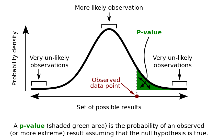
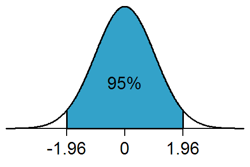
Same calculations may be used to compute a related concept - confidence interval of \(\hat{\theta}\). Confidence interval is an interval that intuitively approximates the likely range in which the parameter \(\theta\) really lies. In our example, the interval would be \(\hat{\theta} \pm 1.96 \hat{\sigma}\), because \(\hat{\theta}\) is normally distributed.

A correct intepretation of a confidence interval is not that simple:

Were we to repeat an experiment multiple times and under the same conditions, an \(x\%\) confidence interval will contain the true value of the estimated parameter around \(x\%\) of the times, assuming that assumptions about data, like being normally distributed, hold.

Frequentist pitfalls

We started with frequentism, because it is the most popular framework used in science and industry. However its use is a source of controversy. Abuse of frequentist methods is blamed for being a cause of the reproducibility crisis in science and is a constant subject of statements, papers, and blog posts detailing its problems.

Some of these arguments can get quite technical, but they are not abstract. The abuse is so pervasive that there are articles on how a conscientous analysts should run her experiments so that she doesn’t get fired by a boss who couldn’t care less about rigor.⁴

However, I’d like to focus on one specific point:

We usually don’t want the answers that frequentism gives.

Perhaps the most damning point for the frequentism and significance testing marriage are not their pitfalls and interpretability problems, but the fact that it’s not really what we want to do. I am particularly fond of this tongue-in-cheek Venn diagram illustrating the point.

For example, consider the definition of a confidence interval. I think it is a rather rare occurance when someone wants to know how would \(95\%\) of experiments that are never run look like. More often than not, we want to know possible values of the parameter under test. The definition is so unnatural that majority of professional researchers hold incorrect beliefs about it.

Even the premise, quantify the surprise of seeing the data under null hypothesis, is under attack. Some argue that proof by contradiction doesn’t quite work when probabilities are involved.

Bayesian approach

A good way to address intepretation problems of frequentist methods is to start asking our questions in the right order. What is the probability of the interesting hypothesis, e.g. B is more effective than A, given data? This kind of problem statement is typical for Bayesian methods. In Bayesian methodology the nature of probability is assumed to be a belief about likelihood of events. Bayesian statistical methods are meant to take into account our beliefs and update them according to data; for example, we visit a casino, strongly believing that their dice are fair, but if a casino dice lands on one 20 times in a row, then a belief about its fairness should decrease.

Bayesian methodology introduces two key concepts. The first is a prior, an initial distribution of the model-under-test’s parameters. Often, it is interpreted as our beliefs running the experiment, but this interpretation can be bent to fit into other use-cases. The second is the eponymous Bayes rule, a mathematical theorem allowing calculation of the posterior: hypothesis’ probability given prior and likelihood:

\[\text{posterior probability: } P(\text{Hypothesis}|\text{Data}) = \frac{P(\text{Data}|\text{Hypothesis})P(\text{Hypothesis})}{P(\text{Data})}\]

Note that \(P(\text{Data}\vert \text{Hypothesis})\) is the value that is calculated in frequentist statistic.

A/B testing

Let’s see how these concepts work out for A/B testing. First we have to agree on a prior. Usually, we don’t know much, so we might as well assign uniform probability distribution to \(\theta_A, \theta_B\). By applying the Bayes rule to experimental data, which consists of numbers of successes and attempts in each variant, we’ll get the posterior probability distribution of variants’ parameters. In our case the posterior probability distribution is conveniently expressible by a Beta distribution. If you’d like to understand what happens under the hood, then I recommend an excellent introductory series “Understanding empirical Bayes estimation (using baseball statistics)”.

With the probability distribution we can do all kinds of stuff we couldn’t do with frequentist methodology. Like plot its density:

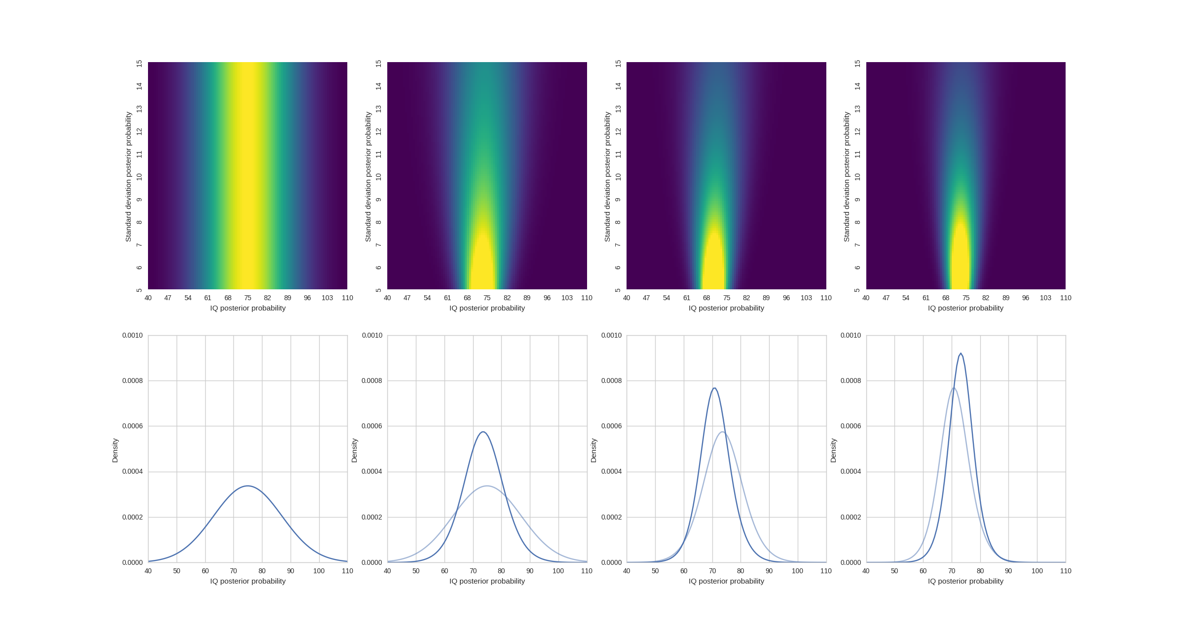An example of how the Bayes rule updates the underlying prior from bobs-iq

As for our website’s design testing, we may, for example, plot the distribution of the absolute difference between conversion rates \((\theta_B - \theta_A)\):

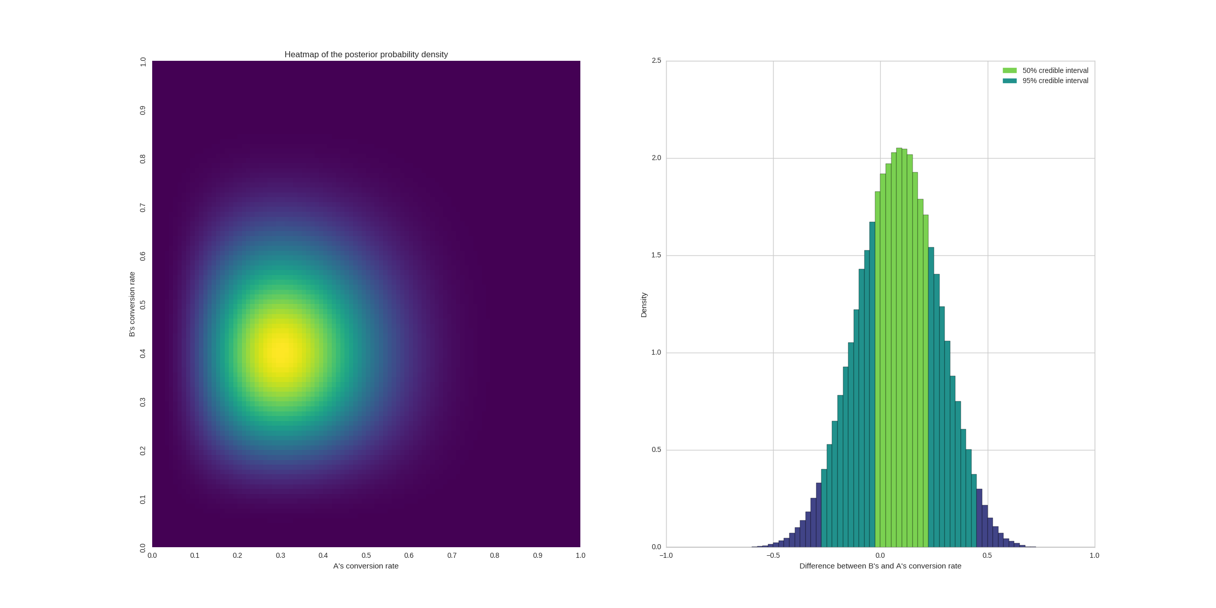Posterior probability when each group has 10 samples. B has 4 conversions and A has 3.

In the plot, I have colored two credible intervals - a Bayesian analogue of confidence interval but with a more palatable interpretation:

With \(95\%\) chance, the expected value is in the credible interval.

And the intepretation plight never appears.⁵

Multi-armed bandit problem - using Bayesian method to minimize loss

Returning a posterior probability opens a world of possibilities for choosing an experiment’s goal. So far, I have presented a basic goal - finding out the probability that B is better than A. I’d like to show one other popular approach that shows how flexible a Bayesian method can be - minimizing the expected loss. For example, imagine a drug trial where we compare two drugs with each other. In our case, we might want to focus on minimizing patients’ suffering instead of just finding drugs’ relative success rate. Let’s say that during a course of an experiment, data seems to suggest that A is better B, but it’s still not close to certain. Even so, since we suspect that A is better than B, then we should perhaps apply A to more than \(50\%\) of our patients in order to benefit from this knowledge. That is what we mean by minimizing loss. At any given time we only have probability estimates of the expected payoff, and we need to decide whether to assign the next patient to A or B (unlike the previous methods, which assigned randomly). Experiments need to continuously balance exploration (choosing alternative variants in order to learn more about payoffs) and exploitation (choosing the variant we believe to be the best) in order to minimize the expected loss - patient is assigned the worse treatment.

Experiments using this approach are called Multi-armed bandit experiments⁶. The multi-armed bandit problem generalizes the outlined approach to multiple variants with unknown payoff.

Summary

Statistical methods are not used in a vacuum and are usually practiced with a specific purpose in mind. That’s why, the first decision we have to make is not, which statistical method we use, but what are we trying to achieve. Be it decide on an action that will be wrong less than 5% of times, determine a success rate difference between two variants, or minimize expected loss, the goal is what drives the experiment, not the other way around. Also, I heartily recommend using Bayesian methods in your experiments, quite often they are the methods you really need, and they suffer from less caveats than frequentist ones do.

1. A quick search for “best test” or “best estimator” on stats.stackexchange.com or reddit.com reveals many entries. Strictly speaking, there is no such thing as “the best test” or “the correct test” in statistics, since any test and any test evaluation rely on some assumptions. “Understanding Statistics and Statistical Myths” explains this point more thoroughly in the third myth: “[The formula] is the Correct Formula for Sample Standard Deviation.”. ↩

2. Although models are often criticized for not being accurate representations of reality, I would argue that models should be first and foremost useful. Being useful is very much related to being accurate but they are not the same. “All models are wrong but some are useful”. ↩

3. The hat symbol means that given value is an estimate based on a sample. A symbol without a hat is meant to represent a parameter, the true value for the population. ↩

4. “Most winning AB test results are illusory” discusses other commonly occuring mistakes done in A/B testing. ↩

5. You can sometimes hear an argument that Bayesian prior makes statistics subjective with the hidden assumption that subjectivity is bad. I don’t think that the argument or even the hidden assumption are valid. Both approaches are subjective. While frequentism doesn’t offer the degree of freedom in the form of a prior, it makes up for it in other aspects like choice of what constitutes unseen data. This post and the post it links to talk a bit more about it. This Wagenmakers’ paper is an excellent, more in-depth resource to learn more about this issue as well as other matters connected to bayesian-frequentist debate. ↩

6. Funny quote from the article: “Originally considered by Allied scientists in World War II, it [the problem] proved so intractable that, according to Peter Whittle, the problem was proposed to be dropped over Germany so that German scientists could also waste their time on it.”. ↩