Early high-level programming languages
This post will summarise history of the early programming languages as written in Knuth’s article “The early development of programming languages”. Most of the work in this post was done by him.
It is interesting to study the history of computer science, to see how many ideas which are now internalised and taken for granted were then formed in great pains. Even today most accounts on early computer languages skip from assembly languages to FORTRAN, which first appeared in a primitive form in 1954, leaving almost a decade of research in obscurity.
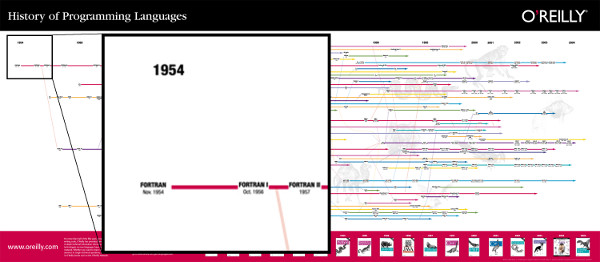 O’reilly’s programming language history skips an entire decade.
Throughout our journey I will present an implementation of the following simple program (called TPK) in each of those languages as it would have been implemented by their authors. Often when an author would have used subscript for their variables, e.g. \(b_i\), I will write b[i] due to limitations of my typesetting engine.
1
2
3
4
5
6
7
8
9
10
11
a = [0.0] * 11
f = lambda t: sqrt(abs(t)) + 5 * t**3
for i in range(11):
  input(a[i])

for i in range(11, -1, -1):
  y = f(a[i])
  if y > 400:
    print(i, "TOO LARGE")
  else:
    print(i, y)
Most languages won’t be able to express this program exactly. Some only handled integers, if so then we will assume that all functions take integers as input and produce them as output. For example sqrt(x) gives the largest integer which square is equal or less than x. If the language does not handle strings then it will output 999 instead of “TOO LARGE”. If the languages does not provide I/O at all then we will assume that input is stored in table a and output will be stored in b[0..21], where b[0], b[2], ... will store i values and odd indexes will store f(a[i]) or 999.
Theoretical languages
Plankalkül - Karl Zuse
Have you ever noticed a growth in your productiveness when your internet access is cut off? I guess that what must have happened to Konrad Zuse, German computer pioneer and engineer, who had been building a relay computer since 1936. Due to heavy Allied bombing of Germany in the ’40s he and his team had lost most of their equipment. He had miraculously saved a Z4 computer and moved to a small Alpine village where he continued his work, but couldn’t really do much with his computer. Therefore he spent his time on theoretical studies leading to design of Plankalkül, a high-level language for a computer, but without much regard whether that language would ever be implemented and how. His language was very comprehensive and contained a lot of ideas that would not appear for a long time afterwards. Using it’s high-level nature Zuse was able to write many complicated programs that were never before written. A notable, not purely algorithmic, example would be a program that played chess. Its source code took 49 pages of manuscript.
Our little algorithm would look like this:
 Plankalkül
Line 1 of this code is the declaration of a compound data type. This is one of the greatest strengths of the Plankalkül. None of the languages we will present had this perceptive notion of data. At the foundation of Zuse’s data system stands a single bit \(SO\) whose value was either “-“ or “+”. Given any sequence of types we could define a compound data type \((\sigma_0, \ldots, \sigma_k)\). Arrays are also available and are defined as \(m \times \sigma\) meaning array of size \(m\) with elements of type \(\sigma\). Furthermore \(m\) could be \(\square\) meaning a list of variable length. Integer variables are represented as \(A9\) and floating points as \(A \triangle 1\).
Lines 2 through 7 define function \(f(t)\) and lines from 8 to 22 define the main program. In Zuse’s language each operation spans multiple lines, for example 11 through 14. The second line of each group identifies subscripts for quantities on the top line. Operations are done mostly on output variables \(R_k\), input variables \(V_k\) and intermediate variables \(Z_k\). The K line denotes components of a variable so for example
\[\begin{array}{c} R\\ 0\\ i\\ \end{array}\]denotes i’th component of \(R_0\).
Zuse used \(\Rightarrow\) symbol for assignment operation. Natural today, this was an important leap from mathematical thinking at the time, where most operations were represented by function composition. The language also has integer for-loops (\(W2(11)\) on 11’th line) and conditionals \(\underset{\cdot}{\rightarrow}\). Zuse made it a point to state mathematical relations between the variables, which we would now call invariants.
Many of Zuse’s ideas were far ahead of his times and would not appear until late ’50s or early ’60s, especially expressive and hierarchical data structures. The reasons for this are twofold. Firstly the hardware at the time wasn’t powerful enough to implement this language in an efficient manner. Zuse tried doing so:
but this project necessarily foundered the expense of implementing and designing compilers outstripped the resources of my small firm. [Konrad Zuse]
Lastly his work lived in relative obscurity and few language designers were aware of it.
Flow diagrams
On the other side of the Atlantic, two famous mathematician’s, Goldstine and von Neumann, tackled the problem or representing algorithms in a precise and readable way. They used a pictorial representation, which would later be dubbed a flowchart. Despite some differences it should be familiar to modern computer scientists.
 Flowchart
Flowcharts consisted of four parts. Operation boxes, marked with Roman numerals, contained operations in a form of assignments to memory locations. Alternative boxes, also marked with Roman numerals, represented a branch operation with two exits \(+, -\) chosen based on the quantity in the box. Substitution boxes, marked with a # and using a \(\rightarrow\) symbol, meant a change in notation. This is an important remark, they did not represent any physical machine operation. Lastly there were also assertion boxes connected to arrows with a dashed line, they contained invariants which were guaranteed by the algorithm.
The flowchart was meant to be a tool used in designing a correct program, which would later be translated to a machine code by a programmer. Therefore it could contain some curiosities coming from machine design. For instance, the example program uses scaling. It assumes that a machine contains 40-bit words which represent a number \(-1 \leq i < 1\), therefore to represent a different range it is necessary to scale it by multiplication by \(2^{i}\).
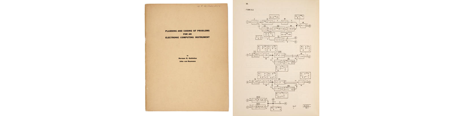 Goldstine and von Neumann’s beautifully typeset book
Unlike Zuse’s Plankalkül, Flowchart was well-known, thanks to von Neumann’s prestigious name and their effort in typing and distributing their work among computer scientist at the time. Notice that it didn’t contain any idea of a function (our \(f(t)\) function had to be inlined) or for-loops or different data types.
Curry — a logician’s approach
Haskell B. Curry, whose name was used to name the Haskell language, worked in Naval Ordnance Laboratory and wrote two lengthy memoranda, which were never published, about his approach to program representation. His experience in writing large programs for ENIAC suggested him a more compact notation than Flowchart uses.
His aims, which today would be similar to aims of structural programming, were quire laudable:
The first step in planning the program is to analyse the computation into certain main parts, called here divisions, such that the program can be synthesised from them. Those main parts must be such that they, or at any rate some of them, are independent computations in their own right, or are modifications of such computations. [Haskell Curry]
Unfortunately in practice his proposal was not successful, because the way he factored the problem was not very natural and his solutions tended to be very complicated.
\(\begin{eqnarray} F(t) &=& \left\{\sqrt{|t|} + 5t^3:A\right\}\\ I &=& \{10:i\} \rightarrow \{t = L(a+i)\} \rightarrow F(t) \rightarrow \{A:y\} \rightarrow II \rightarrow It_7(0,i) \rightarrow O_1 \& I_2\\ II &=& \{x = L(b + 20 - 2i)\} \rightarrow \{i:x\} \rightarrow III \rightarrow \{w = L(b + 21 - 2i)\} \rightarrow \{y:w\}\\ III &=& \{y > 400\} \rightarrow \{999:y\} \& O_1 \end{eqnarray}\)
One of the complexities of this language is that components may have multiple entries and exits.
\(\{E:x\}\) means compute value of E and put it into location x.
A denotes the accumulator of the machine.
\(\{x = L(E)\}\) means compute value of E and substitute it into all appearances of x.
\(X \rightarrow Y\) means substitute instruction group Y for the first exit of X.
\(I_j, O_j\) denote the j’th entrance and exit of given instruction group.
\(\{x > y\} \rightarrow O_1 \& O_2\) means if \(x > y\) go to \(O_1\), otherwise go to \(O_2\).
\(It_7(m,i) \rightarrow O_1 \& O_2\) means decrease \(i\) by 1 and if \(i \geq m\) then go to \(O_1\) or else go to \(O_2\).
What’s unique about his work is that he gave recursive description of a procedure to convert generic arithmetic expressions into a machine code. In other words he was the first person to describe the code-generation phase of a compiler. For example the program he would have generated for \(F(t)\) would like this:
\[\begin{eqnarray} \{|t| : A\} &\rightarrow& \{\sqrt{A} : A\} \rightarrow \{A:w\} \rightarrow \{t : R\} \rightarrow \{tR : A\} \rightarrow \{A:R\}\\ &\rightarrow& \{tR:A\} \rightarrow \{A:R\} \rightarrow \{5R:A\} \rightarrow \{A+w: A\}\\ \end{eqnarray}\]Practical languages
Short Code
The previously discussed languages were purely theoretical in nature. They were never implemented until recent times and existed purely as help in program design. It was the programmer’s job to translate them into machine code. We now turn our attention to languages which were practically used.
The title of the first high-level language to be actually implemented goes to Short Code. It was suggested by John W. Mauchly, the engineer behind ENIAC, in
- It wasn’t an instant success, despite its historical significance, which is not surprising. Short code was implemented for UNIVAC, and there were very few UNIVAC users. Also short code was an algebraic interpreter, it interpreted the code at 50:1 performance ratio. In times when computer time was extremely valuable, while programmers were treated like Hitchcock treated his actors, this was unacceptable to many.
Let’s get to see some code:
1
2
3
4
5
6
7
8
9
10
11
12
13
14
15
16
17
18
19
20
21
22
23
Memory equivalents: i = W0, t = T0, y = Y0
Eleven inputs go respectively into words: U0, T9, ..., T0
Constants: Z0 = 000000000000
           Z1 = 010000000051 [1.0 in decimal form]
           Z2 = 010000000052 [10.0]
           Z3 = 040000000053 [400.0]
           Z4 = △△△TOO△LARGE
           Z5 = 050000000051 [5.0]
Equation number recall information [labels]:
           0 = line 01, 1 = line 06, 2 = line 07

Short Code:
00     i = 10
01  0: y = (√ abs t) + 5 cube t
02
03     y 400 if≤to 1
04     i print, 'TOO LARGE' print-and-return
05     0 0 if=to 2
06  1: i print, y print-and-return
07  2: T0 U0 shift
08     i = i - 1
09     0 i if≤to 0
10     stop
Surprisingly it is very readable, but a few quirks need to be explained. First of the short code interpreter used coded representation form, a kind-of byte code, and UNIVAC used twelve 6-bit bytes. Therefore the line 01 had to be split into two. Also there were no subscripted variables, but it had a shift operation which performed a cyclic shift in a specified block of memory. For instance, line 07 means:
1
temp = T0, T0 = T1, ..., T9 = U0, U0 = temp;
Intermediate Programming Language - Burks
Independently from Short Code, as many of this stuff was done, Arthur Burks and his colleagues tried to simplify the job of coding. Their effort was to transform “Ordinary Business English” description of a data-processing problem to the more precise “Internal Program Language”.
This has two principal advantages. First, smaller steps can more easily be mechanised than larger ones. Second, different kinds of work can be allocated to different stages of the process and to different specialists. [Arthur W. Burks]
Like Plankalkül it uses right-hand assignment.
1
2
3
4
5
6
7
8
9
10
11
12
13
14
15
16
17
18
19
20
21
22
23
24
    1.  10 → i
To 10.

From 1,35
    10. A+i → 11              Compute location of a[i]
    11. [A+i] → t             Look up a[i] and transfer to storage
    12. |t|**(1/2) + 5t^3 → y y[i] = sqrt(abs(a[i])) + 5a[i]^3
    13. 400,y; 20,30          Determine if v[i] = y[i]
To 20   if y > 400
To 30   if y ≤ 400
From 13
    20. 999 → y               v[i] = 999
To 30
From 13,20
    30. (B+20-2i)' → 31       Compute location of b[20 - 2i]
    31. i → [B+20-2i]         b[20-2i] = i
    32. (B+20-2i) + 1 → 33    Compute location of b[21 - 2i]
    33. y → [(B+20-2i)+1]     b[21-2i] = v[i]
    34. i-1 → i               i → i + 1
    35. i,0; 40, 10           Repeat cycle until i negative
To 40   if i < 0
To 10   if i ≥ 0
From 35
    40. F                     Stop execution
The ‘ symbol that appears in line 30. meant that the computer was to save this intermediate result.
Again, even the author feels it is necessary to write an apology about its inefficiency and suggests that it might be useful for design.
It should be emphasized, however, that even if it were not efficient to use a computer to make the translation, the Intermediate PL would nevertheless be useful to the human programmer in planning and constructing programs. [Burks]
It is worth noting that Burks was a mathematician and he has developed a mathematical notation for writing programs, however, as most mathematicians do, he resigned after discovering huge reluctance to even use mathematical symbols.
I used to be mathematics professor. At that time I found there were a certain number of students who could not learn mathematics. I then was charge with a job of making it easy for businessmen to use our computers. I found it was not a question of whether they could learn mathematics or not, but whether they would. … They said, “Throw those symbols out – I do not know what they mean, I have not time to learn symbols.” I suggest a reply to those who would like data processing people to use mathematical symbols that they make them first attempt to teach those symbols to vice-presidents or a colonel or admiral. I assure you that I tried it.
Rutishauser’s first compiler
As it is usually the case with Europe, it was more concerned with research than with business. Z4 relay computer, the same model that was built by Konrad Zuse, had been rebuilt and worked in the Swiss Federal Institute of Technology. Heinz Rutishauser was working with that machine, and although his main functions were not connected to programming, as he himself said:
I had to do other work – to run practically single-handed a fortunately slow computer as mathematical analyst programmer, operator and even troubleshooter. [Rutishauser]
he published a treatise in 1952, describing a hypothetical computer and a simple algebraic language together with two compilers for that language.
1
2
3
4
5
6
7
8
1 Für i = 10(-1)0
2 a[i] ⇒ t
3 (Sqrt Abs t) + (5 x t x t x t) ⇒ y
4 Max(Sgn(y-400), 0) ⇒ h
5 Z O[i] ⇒ b[20 - 2i]
6 (h x 999) + ((1-h) x y) ⇒ b[21 - 2i]
7 Ende Index i
8 Schluss
The language is restrictive. The only control structure it contains is a very crude for loop. Since there are no unconditional jumps, let alone if branches, to implement TPK’s decision Rutishauser’s code would have to use mathematical functions like Max, Sgn (lines 4 and 6). Another problem is that there is no easy mechanism to switch between indices and other variables. Indices were completely tied to Für-Ende loops. Therefore the example program invokes a trick on line 5. Z O[i] is intended to use the Z instruction which transfered an indexed address to the accumulator in Rutishauser’s machine.
As with Short Code, the source code had to be transliterated and the programmer had to allocate storage for variables and constants.
Böhm dissertation - first compiler written in compiled language
Corrado Böhm, an Italian graduate student, developed his own machine, language and translation mechanism in 1950 and published in 1952. It must be noted that he had only known about Zuse’s and von Neumann’s results and had developed in complete independence from Rutishauser. Böhm’s distinctive contribution is that he wrote his compiler in his own language.
The language itself has a special elegance to it, because every operation is a form of an assignment. The compiler is also remarkable for its brevity. It took only 114 lines of code, 59 for decoding expressions with parentheses, 51 for decoding and 4 for deciding between those two cases. His parsing technique was also faster, it took around \(\left(O(n)\right)\) time as opposed to Rutishauser’s \(O\left(n^2\right)\)
1
2
3
4
5
6
7
8
9
10
11
12
13
14
15
16
17
18
19
20
21
22
23
24
25
26
27
28
29
30
31
32
33
34
35
36
37
38
39
40
41
42
43
44
45
46
47
48
49
50
51
52
53
54
55
56
57
58
59
A. Set i = 0 (plus the                                π → G
   base address 100 for                             100 → i
   the input array a).                                B → π

B. Let a new input a[i] be                           π' → B
   given. Increase i by unity,                        ? → ↓i
   and proceed to C if i > 10,                      i+1 → i
   otherwise repeat B.  [(1∩(i∸110))∙C]+[(1∸(i∸110))∙B] → π

C. set i = 10.                                       π' → B
                                                    110 → i

D. Call x the number a[i],                           π' → D
   and prepare to calculate                          ↓i → x
   its square root r (using                           E → X
   subroutine R), returning                           R → π
   to E.

E. Calculate f(a[i]) and                             π' → E
   attribute it to y.                      r+5∙↓i∙↓i∙↓i → y
   If y > 400, continue [(1∩(y∸400))∙F]+[(1∸(y∸400))∙G] → π
   at F, otherwise at G.

F. Output the actual value                           π' → E
   of i, then the value                           i∸100 → ?
   999 ("too large").                               999 → ?
   Proceed to H.                                      H → π

G. Output the actual                                 π' → G
   values of i and y.                             i∸100 → ?
                                                      y → ?
                                                      H → π

H. Decrease i by unity,                              π' → H
   and return to D if                               i∸1 → i
   i≥0. Otherwise stop. [(1∸(100∸i))∙D]+[(1∩(100∸i))∙Ω] → π


R. Set r = 0 and t = 2^{46}                          π' → R
                                                      0 → r
                                         70368744177664 → t
                                                      S → π

S. If r+t ≤ x, go to T,                              π' → S
   otherwise go to U.                             r+t∸x → u
                                    [(1∸u)∙T]+[(1∩u)∙U] → π

T. Decrease x by r+t,                                π' → T
   divide r by 2, increase                        x∸r∸t → x
   r by t, and go to V.                           r:2+t → r
                                                      V → π

U. Divide r by 2.                                    π' → U
                                                    r:2 → r
                                                      V → π

V. Divide t by 4. If t = 0,                          π' → U
   exit, otherwise return to S.                     t:4 → t
                                    [(1∸t)∙X]+[(1∩t)∙S] → π
As said earlier every operation is an assignment. π is a program counter so B → π means go to B. Statement π' → B means this is label B. A loading routine preprocesses the code to set the value of this variable. The symbol ? is used for I/O in an obvious manner. ↓ is used for indirect addressing so ?→↓i means read input to memory location pointed by i.
Böhm machine only had non-negative integers of 14 decimal digits length. Therefore he used logician’s subtraction operator ∸:
\[x ∸ y = \left\{ \begin{array}[rl] (x - y & x > y\\ 0 & x\leq y\end{array}\right.\]Set intersection operator \(\cap\) meant minimum operation. Although Böhm’s language had a goto operation, still there was no branching as in Rutishauser’s, therefore one had to resort to mathematical tricks to get it.
AUTOCODE - first real compiler
Notice that so far we have seen no compiler that has actually been implemented on a real machine. Such a thing would be created by Alick E. Glennie for the Manchester Mark I machine in late 1950’s. Perhaps the reason why it was that this particular machine saw the first real compiler is due to its complexities and intricacies. Its machine language made programming by hand hard enough that an engineer though the benefits of a compiler outweigh the cost of performance. Here is how Glennie stated his motivations at a lecture in 1953:
The difficulty of programming has become the main difficulty in the use of machines. Aiken has expressed the opinion that the solution of this difficulty may be sought by building a coding machine, and indeed he has constructed one. However it has been remarked that there is no need to build a special machine for coding, since the computer itself, being general purpose, should be used. … To make it easy, one must make coding comprehensible. This may be done only by improving the notation of programming. Present notations have many disadvantages: all are incomprehensible to the novice, they are all different (one for each machine) and they are never easy to read. It is quite difficult to decipher coded programmes even with notes, and even if you yourself made the program several months ago.
As we can see the problems with readability and programmer’s short memory are ubiquitous.
1
2
3
4
5
6
7
8
9
10
11
12
13
14
15
16
17
18
19
20
21
22
23
24
25
26
27
28
29
30
31
32
33
1  c@VA t@IC x@½C y@RC z@NC
2  INTEGERS +5 →c
3        →t
4     +t     TESTA Z
5     -t
6            ENTRY Z
7  SUBROUTINE 6 →z
8    +tt →y →x
9    +tx →y →x
10 +z+cx   CLOSE WRITE 1

11 a@/½ b@MA c@GA d@OA e@PA f@HA i@VE x@ME
12 INTEGERS +20 →b +10 →c +400 →d +999 →e +1 →f
13 LOOP 10n
14    n →x
15 +b-x →x
16    x →q
17 SUBROUTINE 5 →aq
18 REPEAT n
19   +c →i
20 LOOP 10n
21  +an SUBROUTINE 1 →y
22  +d-y TESTA Z
23  +i SUBROUTINE 3
24  +e SUBROUTINE 4
25           CONTROL X
26           ENTRY Z
27  +i SUBROUTINE 3
28  +y SUBROUTINE 4
29           ENTRY X
30  +i-f →i
31  REPEAT n
32  ENTRY A CONTROL A WRITE 2 START 2
A look at this code and the fact that this was done to simplify Mark 1’s machine language can give a sense of how complicated the machine language really was. This language is still very machine dependent. Lines 1-10 represent a subroutine for calculation of f. CLOSE WRITE 1 says the the preceding lines constitute subroutine number 1. WRITE 2 START 2 says that the preceding line constitute subroutine 2 and program should start its execution from that subroutine.
Programmer had to assign storage for variables, as with most previous languages, this is done in lines 1 and 11. Glennie shied from using constants so his language has been extended here with INTEGERS instruction. Originally there was only FRACTIONS for constants in range \(\left[-\frac{1}{2}, \frac{1}{2}\right]\), but since scaling was so complicated it was omitted from the code.
At the beginning of subroutine 1 its argument is in the lower accumulator. Line 3 assigns it to variable t. Line 4 is an if branch and means: “Go to label Z if t is positive”. Line 5 puts -t in the accumulator. Line 6 defines label Z. Line 7 applies subroutine 6 (square root) to lower accumulator and stores it in z. On line 8 we compute the product of t by itself which fills both upper and lower accumulators and the upper part, which is assumed to be zero, is stored in y. Finally line 10 completes the calculation of \(f(t)\) by leaving \(z+5x\) in the accumulator. The CLOSE operator causes the compiler to forget the meaning of label Z, but the machine addresses of c, x, y, and z remain.
Line 11 introduces new storage assignments, and reassigns addresses of c and x. Line 13 through 18 form the input loop, n being an index register of Mark I; other indexes are: k, l, n, o, q, r. Loops are always done for decreasing values up to and including 0. Lines 14 through 16 set q to \(20 - n\). The compiler recognised conversions between index and normal variables by insisting that all other algebraic statements begin with + or - sign. Line 17 says to store the result of subroutine 5 to \(a_q\).
The main loop is between lines 20 and 31. Line 21 applies function \(f(t)\) to \(a_n\) any puts the result into accumulator. Lines 23,24,27, and 28 print the result. CONTROL X is an unconditional jump to label X.
ENTRY A CONTROL A define an infinite loop, this was a sort of dynamic stop used to terminate a computation in Mark 1.
That is all that is required to understand essentials in Glennie’s AUTOCODE. One noteworthy thing about his compiler is that according to him the loss of efficiency is in the range of 10%. Narrowing the performance gap between a compiler and human programmer.
Unfortunately his papers were never published due to secrecy of British atomic weapons project and few of Manchester’s users used his work. Also he wasn’t a resident at Manchester, so he couldn’t advertise well enough, and automatic programming wasn’t an issue of importance back then. In 1965 Glennie remarked:
[The compiler] was a successful but premature experiment. Two things I believe were wrong: (a) Floating-point hardware had not appeared. This meant that most of a programmer’s effort was in scaling his calculation, not in coding. (b) The climate of thought was not right. Machines were too slow and too small. It was a programmer’s delight to squeeze problems into the smallest space. …
I recall that automatic coding as a concept was not a novel concept in the early fifties. Most knowledgeable programmers knew of it, I think. It was a well known possibility, like the possibility of computers playing chess or checkers. … [Writing the compiler] was a hobby that I undertook in addition to my employers’ business: they learned about it afterwards. The compiler … took about three months of spare time activity to complete.
The idea of compilers gets some traction
So by the early 1950’s we already have witnessed individual discoveries and inventions which brought interpreters, compilers and some basic structures like subroutines, control statements etc. People were aware that automatic programming existed (nobody called it compiling), but programmers were mostly shying away from it. Assemblers (programs which translate from assembly mnemonics) and libraries (mostly floating-point functions) were enough for most. Ability to express programs more succinctly was the main issue.
However the idea that programs could not just be interpreted, but also translated into machine coded was getting some traction and advocates. Grace Hopper was a particularly active spokesperson for automatic programming during the 1950’s and helped organise two conferences in 1954 and 1956 under the sponsorship of the Office of Naval Research. Although it must be mentioned that the contributions of Zuse, Curry, Burks, Mauchly, Böhm and Glennie were not mentioned at either symposium.
Today we would say the the biggest event at either symposium was the announcement of a system implemented by Laning and Zierler for the Whirlwind computer at M.I.T in 1954. Though you wouldn’t be able to tell by looking at the symposium’s proceedings.
We will skip detailed explanation of the language and rather focus on its impact and its features. First of the language was defined independently from the machine and publisheds manual were written for a novice for the first time.
Their language featured subroutines, basic control structures (no for though), subscripts for variables, operator precedence. They even included a mechanism for integrating a system of differential equations.
Unfortunately all those features turned out to be expensive and the resulting compiler did not optimise well enough, causing too many calls to slow memory subsystem (“the drum”) compared to a program done by hand. The authors reflect that the performance in such scenarios was ten to one. However the system was still used in case a fast solution was required.
FORTRAN 0 - efficient and simple
In early 1954 John Backus assembled a group at IBM destined to work on improved systems of automatic programming. They have learned about Laning and Zierler system and even witnessed its operation. They realised that the big problem facing them was implementing a language with efficiency.
At that time, most programmers wrote symbolic machine instructions exclusively (some even used absolute octal or decimal machine instructions). Almost to a man, they firmly believed that any mechanical coding method would fail to apply that versatile ingenuity which each programmer felt he possessed and constantly needed in his work. Therefore, it was agreed, compilers could only turn out code which would be intolerably less efficient than human coding (intolerable, that is, unless that inefficiency could be buried under larger, but desirable, inefficiencies such as the programmed floating-point arithmetic usually required then). …
[Our development group] had one primary fear. After working long and hard to produce a good translator program, an important application might promptly turn up which would confirm the views of the sceptics: … its object program would run at half the speed of a hand-coded version. It was felt that such an occurrence, or several of them, would almost completely block acceptance of the system.
By the end of 1954, Backus’s group had specified “The IBM Mathematical FORmula TRANslating system, FORTRAN”. Almost all languages after that were named after acronyms. The aim of this specification was to provide a language that would combine the best of both worlds: easy of coding and efficiency.
1
2
3
4
5
6
7
8
9
10
1     DIMENSION A(11)
2     READ A
3  2  DO 3,8,11 J=1,11
4  3  I = 11 - J
5     Y = SQRT(ABS(A(I+1))) + 5*A(I+1)**3
6     IF (400. >= Y) 8,4
7  4  PRINT I,999.
8     GO TO 2
9  8  PRINT I,Y
10 11 STOP
The DO statement means do statements 3 through 8 and then go to 11. IF statement was originally only a two-way branch and the only acceptable relations were =, >, >=. On 5th line we see subroutines calls, their name had to be at least 3 characters long, conversely variable names could be take up to 2 characters, which was an improvement; in all previous languages variables took only a single letter. The GO TO statement did not mean an unconditional jump, but merely indicated a next iteration.
The FORTRAN 0 was also the first language to define its syntax rigorously.
1954 was the date specification and basic implementation release. It took the team 2.5 more years to complete the compiler.
Brooker’s Autocode
Europe was also busy developing practical language implementation. R. Brooker, knowing about AUTOCODE limitations, introduced a much cleaner Autocode, which would be nearly machine independent and would use floating-point arithmetic. Unfortunately, probably due to focus on efficiency, there was no way for user to define functions, only one operation per line was permitted and there were few mnemonic names.
The language was actually realised in 1956 and the Autocode should be easily readable.
1
2
3
4
5
6
7
8
9
10
11
12
13
14
15
16
17
18
19
20
21
    1     n1 = 1
         vn1 = I         reads input into v[n[1]]
          n1 = n1 + 1
       j1,11 ≥ n1        jumps to 1 if n[1] ≤ 11
          n1 = 11
    2    *n2 = n1 - 1    prints i = n[1] - 1
      j3,v12 ≥ 0∙0
         v12 = 0∙0 - v12 sets v[12] = |v[12]|
    3    v12 = F1(v12)   v[12] = sqrt(|a[i]|)
         v13 = 5∙0⊗vn1
         v13 = vn1⊗v13
         v13 = vn1⊗v13   v[13] = 5a[i]^3
         v12 = v12+v13
      j4,v12 = 400∙0
        *v12 = v12       prints y
          j5
    4   *v12 = 999∙0     prints 999
    5     n1 = n1-1
       j2,n1 > 0
             H
           (j1)
The instruction in parenthesis (j1) was not to be compiled, but rather executed immediately. Here it starts the program at label 1.
This language is not really high-level, but one has to admit that it looks cleanly, especially compared to its predecessor. Also its main focus was efficiency of compiled code, especially desire to keep the information flowing between the electrostatic high-speed memory and the drum.
The language was a huge success.
Since its completion in 1955 the Mark I Autocode has been used extensively for about 12 hours a week as the basis of a computing service for which customers write their own programs and post them to us. [Brooker]
FORTRAN I - The end of our journey
During the ’50s the ongoing effort on FORTRAN was widely publicised and although still the were doubts whether such a thing was feasible the following quote perhaps sums up the attitude:
As far as automatic programming goes, we have given it some thought and in the scientific spirit we intend to try out FORTRAN when it is available. [Goldstein, 1956]
On October 1956 the first manual was published. Beautifully typeset and written, it announced that the hand-written programs will be as efficient as those done manually and the release of FORTRAN will happen in late 1956.
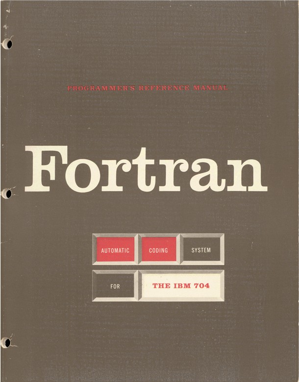 First FORTAN manual cover.
Obviously “Late 1956” was the date for someone sucked in a wormhole as most big software projects go, because the first release didn’t see the daylight until April 1957. It was bug-ridden, had unfinished important parts and often crashed during compilation. Eventually though, it was polished and it became clear that FORTRAN I was working. While there were still critics, who cautioned against using “automatic programming”, as they have decreased utility and efficiency, in reality the share of high-level programming would soar in short time.
1
2
3
4
5
6
7
8
9
10
11
12
13
14
15
16
    C  THE TPK ALGORITHM, FORTRAN STYLE
       FUNF(T) = SQRTF(ABSF(T))+5.0*T**3
       DIMENSION A(11)
    1  FORMAT(6F12.4)
       READ 1, A
       DO 10 J = 1,11
       I = 11-J
       Y = FUNF(A(I+1))
       IF (400.0-Y)4,8,8
    4  PRINT 5, I
    5  FORMAT(I10, 10H TOO LARGE)
       GO TO 10
    8  PRINT 9, I, Y
    9  FORMAT(I10, F12.7)
    10 CONTINUE
       STOP 52525
FORTRAN I implementation of TPK
FORTRAN I had some improvements from FORTRAN 0, mostly: ability to add comments, arithmetic statement functions, formats for I/O, return code (octal number displayed at the STOP instruction).
Summary
This concludes our foray into the programming language archaeology. I have skipped some developments, like early declarative languages or what happened behind the Iron Curtain. We only got the look into the imperative languages path. The path that saw multiple rediscoveries of similar ideas and the struggle with the mindset at the time. An engineer or scientist had to somehow reconcile easiness of coding with the slow machine speed and do this while not knowing what would work and what wouldn’t, which ideas are worth pursuing and which aren’t. It was a very hard task since nobody had ever done this before and what they had seemed good enough then. When complacency is common it is difficult to innovate.