Lessons in writing and testing an audio modem in Python
In one of my current prototype projects I need to encode voice into binary data and then later transfer it through a voice channel. This forced me to push my limits and learn new things which I will describe here. This post will explain technologies I use, rationale behind them, and give basic advice on how to use them. First I will describe basic theory around modulation and demodulation, then I will describe how to combine Cython and profiling to build a flexible and efficient Python application. In the last section I will talk about pulseaudio and how it allows me to perform user testing without using an external device.
Modulation and demodulation
The module that I am building encodes and decodes voice. The encoder has one input: a continuous stream of voice represented by audio samples. On the output it plays audio that is transmitted by an independent voice communicator. The decoder does the reverse.
What makes this task non-trivial is that in the middle the voice is encoded, producing a seemingly random bytestring. This task includes a few challenges:
- How one should modulate the bytestring so that voice communicators do not distort it?
- Given that voice channels have limited capacity how should I encode the human voice so that it fits?
- How can I efficiently demodulate the modulated signal?
Basics of audio signals
The sound that we hear is a result of a mechanical wave of pressure and displacement propagating through air. As such we can represent any sound as a wave. Wave being a continuous signal needs to be discretized to be representable in computer memory and there are two ways to go about it.
First we can represent a wave as a sum of its fundamental frequencies. It is a mathematical fact that:
\[f(x) : [0,1] \rightarrow \mathbb{R}\] \[f(x) = \sum_{i=0}^\infty \left(A_i \sin(ix) + B_i \cos(ix)\right)\]Every continuous function on closed interval can be represented as a (potentially infinite) sum of basic frequencies, that is:
We might keep a table of coefficients \(A_i, B_i\) for all audible frequencies. Humans can hear up to 20kHz, so the size of this table goes up to 20000 thousand for each time frame.
This representation may allow for easier reproduction of signal through mechanical means (combine all those fundamental frequencies and you are done), but is impractical.
The second raw representation uses samples of the wave taken at specified intervals. For example a typical .wav file, which uses this format, stores the amplitude of the wave for every \(\frac{1}{44100}\) part of a second. The frequency of sampling is called a sampling rate. The sampling rate used in telephony is 8000Hz. The reasoning behind the value of the sampling rate will be explained later.
Both representations are equivalent in the sense that one can transform from one to the other. From fundamental frequencies we can produce sampling by simply calculating wave values at given points. To get the other way around we need to use the discrete Fourier transform.
Discrete Fourier transform
Fourier transform is a general mathematical tool which transform a wave function into a function of fundamental frequencies. That is the resulting function maps each of its argument to its power inside the argument. The discrete version of the Fourier transform maps list of samples of the wave to values of fundamental frequencies of the wave that generated them. The formula looks as follows:
\[X_k = \sum_{i=0}^{\left\lceil\frac{N}{2}\right\rceil} x_k e^{-i2\pi k n / N}\]Where \(x_k\) are samples and \(X_k\) is a complex number representing fundamental coefficients in the form of: \(\frac{B_k}{2} + \frac{A_k}{2} i\) if \(k > 0\) and \(X_0 = B_0\). Note that I am using \(\left\lceil\frac{N}{2}\right\rceil\) as the upper limit of the sum instead of often seen \(N-1\). That’s because further numbers do not give any more information.
Naively calculating the DFT takes \(O\left(N^2\right)\) time. Fortunately there exists a fast Fourier transform algorithm which takes \(O\left(N \log N\right)\).
Originally I planned to make an entire post about the transform, but I don’t think I have so much time at hand plus there are obviously much better resources available on the internet. I recommend this site.
The sampling rate that we want is determined by Nyquist-Shannon theorem
If a function x(t) contains no frequencies higher than B Hz, it is completely determined by giving its ordinates at a series of points spaced 1/(2B) seconds apart.
That means that if we want reliably represent frequencies up to B Hz we need have twice that sampling rate. Since telephony was meant to transmit voice and human voice happens in a range up to 300Hz then 8000 sampling rate was more than enough.
Modulating data
We know enough to understand important trade-offs of signal modulation. Our task now is to encode binary data into a voice channel in such a way that the channel’s internal encoding will not distort the signal too much. Here I used Hermes. It’s a research protocol meant to encode data inside telephony. The authors use relative frequency shift keying (RFSK) for modulation. FSK is a modulation technique where we encode each bit as a signal pulse of specific frequency. In Hermes we encode each bit as a relative change of frequency, specifically 0 is a drop in frequency and 1 is a rise. In order to not go outside the voice band we expand each original bit into 01 or 10 sequence. Combined with the fact that the telephony can reliably carry signal only up to 4000 Hz and that each pulse needs to take at least \(\frac{1}{4000}\) of a second this gives as a theoretical maximal throughput of 2000 kbps. Even so authors have achieved sufficient reliability at only 1200 kbps throughput.
The throughput required by telephony to carry voice is 64kbps (8 bits per sample at 8000 samples per second). Comparing it with 1200 kbps, we can get with Hermes, it seems awfully lot and it is. It took me some time to find the state-of-the-art codec which encodes voice with bit rate as low as exactly 1200kbps. Talk about luck. To use it inside Python I had to use Cython to provide a Python interface to codec2. The library is available on my Github. I’m planning on releasing it on PyPi soon.
To be honest I have never used Foreign Function Interface inside any language, which seems weird now. I had tried writing this prototype inside Haskell before, but resigned due to lack of some libraries I would find useful. Now after overcoming my reluctance to FFI I would simply write such a wrapper for Haskell. End of diversion.
Demodulation
So far I have described how the voice is encoded into binary data and how then this data is modulated. We are now left with possibly the most difficult part of the process: demodulation. In the modulation phase we just send samples of pulses of different frequency. So in the demodulation phase we need to do something along the lines of discovering when a pulse begins and what’s its frequency or at least whether it has risen or dropped.
Using FFT
Initially I was ambitious and tried to do it “correctly”. I have researched what kind of method would Digital Signal Processing books propose. I found most methods to be impractical, because they either focused on transforming the signal or seemed to be designed for hardware. In the end I used FFT to generate a spectrogram of input signal. A spectrogram is a result of FFT mapped over time. The simplest way to get a spectrogram is to repeatedly perform FFT over an appropriate window of samples. Additionally that window of samples is multiplied by a Hamming function which is meant to mask any error at the beginning or end of the pulse.
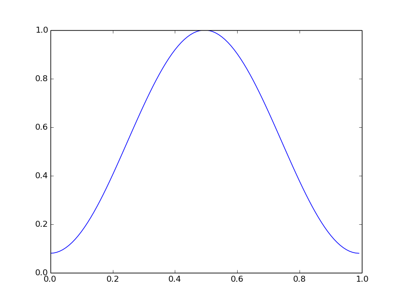 Hamming function
How do I recognize beginning of the pulse? In short I don’t. I sweep the incoming signal and let upper layers check how many errors they get. If the error rate is small then I use that window for decoding until error rate goes up.
Aside from low efficiency of this method it is also inaccurate. At the rate 1200 kbps my base frequency is 2400 Hz. If the sampling rate is 44100 then I get \(\frac{44100}{2400} \approx 18\) samples per window. That means that if I perform FFT on that window then each coefficient is responsible for a frequency window of size \(\frac{44100}{2 \cdot 18} = 1225\). With such a wide window I can not simply find the dominating frequency in the resulting table to demodulate the signal. I need to use some kind weighted sum for comparison.
In the end I decided to abandon this method. It was too imprecise and inefficient. Below I attack a snippet of code performing spectrogram calculation (without some optimizations)
1
2
3
4
5
6
7
8
9
10
11
12
13
14
15
16
17
18
19
20
21
22
23
24
25
26
27
28
29
30
31
32
33
34
35
36
37
38
39
40
41
42
43
44
45
46
47
48
49
50
51
52
def calculateSpectogram(audioSamples
    , frameDuration):
  """Given audio samples and duration of frame in seconds calculate a
  spectrogram matrix. The returning matrix has the result of successive DFTs in
  each column"""
  samples = audioSamples.samples
  sampleRate = audioSamples.sampleRate
  frameSize = round(sampleRate * frameDuration)
  frameCount = round(len(samples) / frameSize)
  cutOffPoint = round(MAX_AVAILABLE_FREQUENCY * frameDuration) + 2
  ftTable = []
  w = np.hamming(frameSize)
  currentFrame = 0
  while round((currentFrame + 1) * frameDuration * sampleRate) <= len(samples):
    begSampleIdx = round(currentFrame * frameDuration * sampleRate)
    endSampleIdx = begSampleIdx + frameSize
    windowedSample = samples[begSampleIdx : endSampleIdx] * w
    ftTable.append(sumFFTTable(np.array(abs(np.fft.fft(windowedSample)))/frameSize))
    ftTable[-1] = ftTable[-1][:cutOffPoint]
    ftTable[-1] = weightedSum(ftTable[-1])
    currentFrame += 1

  return np.array(ftTable)

def generateFrequencyExponent(frequency, sampleCount):
  exponents = np.linspace(0.0, 1.0, sampleCount + 1)[:sampleCount] \
              * 2 * math.pi \
              * frequency \
              * (0.0 + 1.0j)
  return math.e ** exponents

def myFFT(samples, cutOffPoint):
  resultLength = min(len(samples), cutOffPoint)
  result = np.array([0.0] * resultLength)
  for freqIdx in range(resultLength):
    pass

# Two functions below are used for calculating a dominating frequency at
# each window using crude weighted sum

def sumFFTTable(fftTable):
  summedTable = [fftTable[0]]
  for i in range(1, int((len(fftTable) + 1)/2)):
    summedTable.append(fftTable[i] + fftTable[-i])
  return summedTable

def weightedSum(table):
  summed = 0.0
  tableSum = sum(table)
  for (i, elem) in enumerate(table):
    summed += (i  + 1) * elem
  return summed
Zero counting
The most primitive method of estimating frequency is to estimate where the wave function would have cross the zero-value axis and calculate distances between consecutive zeros. This method does not give us distribution of fundamental frequencies and is prone to data and numerical errors. However in this application, since the only thing we need is the relation of frequencies in consecutive frames, it turns out to be quite precise. In fact, more precise than the previous one.
Additionally it is more efficient and fits better into the sweeping framework. We can calculate the differences between zero-crossing beforehand and then perform the sweeping method on the stream of those differences. We avoid performing costly FFT for each missed sample or window.
I can use a simple transformation of input signal to transform it into a wave, or more like a signal from Functional Reactive Programming.
Lesson? Don’t discount simple ideas just because they are primitive.
Now we have an efficient demodulation technique, however Python is not a demon of speed and requires tuning to bring our modem to real-time speed required for voice demodulation. In the next section I will explain how Cython works and how it can greatly improve speed of Python for low cost of just some static type annotations.
Cython
Profiling
The code that I have written was too slow for real-time use. Although I could encode/decode static files, it would happen at 1/5x the speed of audio. I decided to use profiling tools to check what’s the bottleneck. Python’s extensive standard library provides cProfile. It’s a C-extension which makes it more efficient than the pure Python, profile, version. Its use is simple:
1
2
3
cProfile.runctx('self._run()' # Code to run
    , globals() # dictionary of global objects
    , {'self' : self}) # dictionary of local objects
And that’s it. At the end of the run it will print a profiling table, similar to the one below.
1
2
3
4
5
6
7
8
9
10
11
12
197 function calls (192 primitive calls) in 0.002 seconds

Ordered by: standard name

ncalls  tottime  percall  cumtime  percall filename:lineno(function)
     1    0.000    0.000    0.001    0.001 <string>:1(<module>)
     1    0.000    0.000    0.001    0.001 re.py:212(compile)
     1    0.000    0.000    0.001    0.001 re.py:268(_compile)
     1    0.000    0.000    0.000    0.000 sre_compile.py:172(_compile_charset)
     1    0.000    0.000    0.000    0.000 sre_compile.py:201(_optimize_charset)
     4    0.000    0.000    0.000    0.000 sre_compile.py:25(_identityfunction)
   3/1    0.000    0.000    0.000    0.000 sre_compile.py:33(_compile)
This allows for quick identification of program’s bottlenecks.
Now back to the performance problem. Python 3 is slow. It can be up 100 times slower than C source. This is the result of Python’s dynamic typing, primitive values are boxed, objects are dictionaries and function calling requires dynamic dispatch. Statically typed code is simply faster, because it allows the compiler to reason more effectively about the program and therefore required optimizations. Now I recognize 3 general solutions which uses typing to help generate faster code.
- Use statically typed language, but since we don’t want to resign from Python we might code the speed-critical part of code in a faster language and use FFI.
- Use optionally typed language. That is a language that uses optional typing annotation for faster code generation. Note that there are also languages which use optional typing for runtime assertions like Dart.
- Use statically typed language with type inference. See Haskell.
Cython combines 1. and 2. It provides an FFI interface to C libraries and extends language with constructs that help Cython translate quasi-Python code to C. It is really good.
Cython
Cython is a superset of Python which provides FFI to C and C++ and transforms Python code into C with the help of type annotations. Its great strength is that with a few additional keywords it combines the speed of C and Python’s expressiveness.
####.pxd
Cython source code consists of .pxd and .pyx files. .pxd files are basically like C headers and they serve three functions:
- Define which C functions and globals from external libraries should be available in Python’s code.
- Define which Cythons functions should be available through C interface.
- Define C data structures
For example pycodec2 uses codec2.pxd file for codec2 import:
1
2
3
4
5
6
7
8
9
10
11
12
13
14
15
16
17
18
19
20
21
22
23
24
25
26
27
28
29
30
31
32
33
34
cdef extern from 'codec2/codec2.h':
  cdef enum:
    CODEC2_MODE_3200 = 0
    CODEC2_MODE_2400 = 1
    CODEC2_MODE_1600 = 2
    CODEC2_MODE_1400 = 3
    CODEC2_MODE_1300 = 4
    CODEC2_MODE_1200 = 5

  cdef struct CODEC2:
    pass

  CODEC2* codec2_create(int mode)
  void codec2_destroy(CODEC2* codec2_state)
  void codec2_encode(CODEC2 *codec2_state,
      unsigned char * bits,
      short speech_in[])
  void codec2_decode(CODEC2 *codec2_state,
      short speech_out[],
      const unsigned char *bits)
  void codec2_decode_ber(CODEC2 *codec2_state,
      short speech_out[],
      const unsigned char *bits,
      float ber_est)
  int codec2_samples_per_frame(CODEC2 *codec2_state)
  int codec2_bits_per_frame(CODEC2 *codec2_state)
  void codec2_set_lpc_post_filter(CODEC2 *codec2_state,
      int enable,
      int bass_boost,
      float beta,
      float gamma)
  int codec2_get_spare_bit_index(CODEC2 *codec2_state)
  int codec2_rebuild_spare_bit(CODEC2 *codec2_state, int unpacked_bits[])
  void codec2_set_natural_or_gray(CODEC2 *codec2_state, int gray)
Inside pycodec2.pyx we only do:
1
  from codec2 cimport *
and we are done. We can now use those function like if they were Python’s. Here’s an excerpt from pycodec2.pyx:
1
2
3
4
5
6
7
8
9
10
11
12
13
14
15
16
cdef class Codec2: # Our Python's wrapper for Codec2 defined in codec2.pxd
                   # We have to use cdef, because it is a C like struct holding
                   # a C pointer, which pure Python can not.
  '''Wrapper for codec2 state and its functions.

  Initialization method expects an integer defining expected bitrate per
  second.'''
  cdef CODEC2 *_c_codec2_state # C variable contained in this class.
                               # It is inaccessible from pure Python code.

  def __cinit__(self, mode): # Special Cython version of __init__ for C-like
                             # structs. It's called before __init__ and should
                             # be used for initialising C constructs.
    self._c_codec2_state = codec2_create(_modes[mode])
    if self._c_codec2_state is NULL:
      raise MemoryError()
Our Codec2 object partially realizes the second function of .pxd file, because Codec2 is the class that is meant to be used by pure Python code.
Below is an example of a data structure holding audio samples that is implemented with Cython for some speed-up:
1
2
3
4
5
6
7
8
9
10
cdef class AudioSamples:
  cdef public object samples # public means that this field can be accessed by
                             # pure Python code.

  cdef public int sampleRate

  cpdef drop(AudioSamples self, int count) # cpdef means that this function has
                                           # both C and Python interfaces

  cpdef take(AudioSamples self, int count)
As can be noticed, Cython’s provides cdef and cpdef keywords for defining functions with fast C interface, cpdef additionally provides Python’s interface so that it is accessible from purely Python code inside .py files. On default class fields are not accessible from Python’s code unless we provide public or readonly keywords.
####.pyx
The .pyx file is basically a .py file with Cython annotations. Combined with optional .pxd files the Cython generates a .c source code with
1
cython -a signal.pyx
or using automatic build tools in setup.py. The .pyx file is where we can define Python interface for use in pure Python code and also use C libraries and our Cython C functions defined with cdef.
Apart from providing FFI interface, Cython allows for easy optimization using C type annotantion. Transforming
1
2
3
4
def valueAt(self, timeBeg, timeEnd):
  begIndex = findLE(self.waveKeys, self.shift + timeBeg)
  endIndex = findLE(self.waveKeys, self.shift + timeEnd)
  return max(self.waveValues[begIndex : endIndex + 1])
to
1
2
3
4
cpdef float valueAt(self, float timeBeg, float timeEnd):
  cdef int begIndex = findLE(self.waveKeys, self.shift + timeBeg)
  cdef int endIndex = findLE(self.waveKeys, self.shift + timeEnd)
  return max(self.waveValues[begIndex : endIndex + 1])
which is much faster.
Import and build
To use Cython we only have to run:
1
2
import pyximport
pyximport.install()
And later we can just import the module to use Python interfaces defined there.
Inside .pyx files we may also import use C interfaces with cimport command.
Pulseaudio
To test this application we need to transmit the encoded audio into Skype and vice verae while at the same time we use microphone for our modem’s input, but not Skype’s. Linux distributions which use pulse-audio can provide this behaviour.
It provides a sink constructs:
- Sink - single pipe with one sender and multiple listeners. For example a program’s output may be attached toto a sink, which later can be received by other different sinks.
We can set up sink with pactl command line tool:
1
2
3
4
pactl load-module module-null-sink sink_name=SkypeInput sink_properties=device.description="Skype's_Input"
pactl load-module module-null-sink sink_name=SkypeOutput sink_properties=device.description="Skype's_Output"
pactl load-module module-null-sink sink_name=CryptoVoiceInput sink_properties=device.description="CryptoVoice's_Input"
pactl load-module module-null-sink sink_name=CryptoVoiceOutput sink_properties=device.description="CryptoVoice's_Output"
Then when we run our program we can link sink’s and processes’s I/O to respective sinks using pavucontrol.
As a sidenote I’d like to mention that module-loopback may be used to combine streams so that multiple inputs can be mixed.